Graphical LASSO Algorithm

Graphical LASSO Algorithm

GLASSOFAST is the Graphical LASSO algorithm to solve the covariance selection problem.

Consider observations \(X_1, X_2, \dots, X_n\) from multivariate Gaussian distribution \(X\sim \mathcal{N}(0,\Sigma)\). We are interested in estimating the precision matrix \(\Theta = \Sigma^{-1}\).

GLASSOFAST is an efficient GLASS implementation to solve the \(l_1\) regularized inverse covariance matrix estimation problem:

\begin{equation}
arg \underset{X\succ 0}{min}\{-log\ det\ X + tr(SX) + \lambda \sum_{i,j=1}^p |x_{ij}|\}
\end{equation}

where \(x_{ij}\) denotes the \((i,j)\)-th element of matrix \(X\). The \(i\)th columns and rows of matrix \(X\) are denoted by \(\textbf{x}_i\).

This algorithm solves a generalized form of the optimization problem (1), where the regularization term is of the form \(\sum_{ij}\lambda_{ij}|x_{ij}|\).

Here are the loops to realize algorithm:

  • The first loop is controlled by convergence on the whole matrix
  • The second loop iterates through the rows of the matrix
  • The two most inner loops solve a lasso problem for a given row using coordinate descent.

The computation speed of GLASSOFAST is faster than QUIC, GLASSO 1.7 and GLASSO 1.3. Also, the regularization parameter can have large impact on performance.

References

  1. “Sustik, M.A. and Calderhead, B., “GLASSOFAST: An efficient GLASSO implementation,” UTCS Technical Report TR-12-29, November 6, 2012.”
  2. “O. Banerjee, L. E. Ghaoui and A. d’Aspremont, “Model Selection Through Sparse Maximum Likelihood Estimation for multivariate Gaussian or Binary Data,” Journal of Machine Learning Research, 9, pp. 485-516, March 2008.”

Covariance Selection

Covariance Selection

Mean reversion is a classic trading strategy, which assumes that a stock’s price will tend to move to the average price over time. It is a classic indicator of predictability in financial markets.

Traditionally, people use cointegration or canonical correlation analysis to obtain the optimal mean reversion portfolio. However, there are some shortcomings of these methods:

  • The mean reverting portfolios they identify include every asset in the time series analyzed. It involves considerable transaction costs.
  • Less interpretability of the resulting portfolio.
  • Optimally mean reverting portfolios often behave like noise and sometimes vary well inside bid-ask spreads, hence do not form meaningful statistical arbitrage opportunities.

Hence, we want to form portfolios with maximum mean reversion while constraining the number of assets in these portfolios. The covariance selection method is included in this article.

Algorithms for extracting sparse mean reverting portfolios

The asset prices follow a stationary VAR process with

\(S_t = S_{t-1}A + Z_t\)

where \(S_{t-1}\) is the lagged portfolio process, \(A \in R^{n\times n}\) and \(Z_t\) is a vector of i.i.d. \(Z_t\) is the noise term following \(\mathcal{N}(0,\Sigma)\), where \(\Sigma \in S^n\), and it is independent of \(S_{t-1}\). Assume \(S_t\) has zero mean. After computation we get:

\(\hat{A} = (S^T_{t-1}S_{t-1})^{-1}S^T_{t-1}S_t\)

Here are two techniques to get good approximate solutions:

1. Greedy Search

Call \(I_k\) the support of the solution vector \(x\) given \(k > 0\)

\(I_k = \{i \in [1,n]: x_i \neq 0\}\)

by construction \(|I_k| \le k\).

Suppose we have a good approximate solution with support set \(I_k\) given by:

\(x_k = \underset{\{x\in R^n:x_{I^c_k}=0\}}{argmax}\frac{x^TAx}{x^TBx}\)

where \(I_k^c\) is the complement of the set \(I_k\). We seek to add one variable with index \(i_{k+1}\) to the set \(I_k\) to produce the largest increase in predictability by scanning each of the remaining indices in \(I_k^c\). The index \(i_{k+1}\) is then given by:

\(i_{k+1} = \underset{i \in I_k^c}{argmax}\underset{\{x\in R^n:x_{J_i}=0\}}{max}\frac{x^TAx}{x^TBx},\) where \(J_i = I_k^c \setminus \{i\}\)

which amounts to solving  generalized eigenvalue problems of size . We then define:

\(I_{k+1} = I_k\cup \{i_{k+1}\}\)

And repeat the procedure until \(k=n\).

2. Semidefinite Relaxation Techniques

Transfer the original question to the weak convex constraint question:

Maximize \(Tr(AY)\)

Subject to \(1^T|Y|1 – kz \le 0\)

\(Tr(Y) – z = 0\)

\(Tr(BY) = 1\)

\(Y \succeq 0\)

where \(Y = \frac{X}{Tr(BX)}\) and \(z = \frac{1}{Tr(BX)}\).

The computational complexity of this relaxation is significantly higher than that of the greedy search algorithm.

Parameter Estimation

Both \(\Gamma\) and \(A\) estimates suffer from the stability issues. We can penalize the covariance estimation using a multiple of the norm of \(\Gamma\) to stabilize the estimation.

1. Covariance Selection

We estimate the covariance matrix  by maximum likelihood:

\(\underset{X}{max}\ log\ det X – Tr(\Sigma X)-\rho Card(X)\)

where \(Card(X)\) is the cardinality of \(X\), i.e. the number of nonzero coefficients in \(X\) and \(\rho > 0\) is a parameter controlling the tradeoff between likelihood and structure.

The advantages of this process are:

  • Improves the stability of this estimation procedure by implicitly reducing the number of parameters
  • Directly highlights structure in the underlying model.

However, the cardinality penalty makes this problem very hard to solve numerically. So we improve it by:

\(\underset{X}{max}\ log\ det X – Tr(\Sigma X)-\rho \sum_{i,j=1}^n |X_{ij}|\)

2. Estimating Structured VAR Models

(1) Endogenous dependence models

Assume that the conditional dependence structure of the assets \(S_t\) is purely endogenous, with the VAR model \(S_t = S_{t-1}A + Z_t\) where \(Z_t \sim \mathcal{N}(0,\sigma I)\) and choosing \(\sigma\) small enough, we can get \(A\) as a matrix square root of \((I-\sigma\Gamma^{-1})\).

(2) Exogenous dependence models

Modify the previous \(\hat{A} = (S^T_{t-1}S_{t-1})^{-1}S^T_{t-1}S_t\) estimation in order to get a spare model matrix \(A\), we get the columns of \(A\) by solving:

\(a_i = \underset{x}{argmax}||S_{it} – S_{t-1}x||^2 + \gamma ||x||_1\)

3. Canonical Decomposition with Penalized Estimation

We want to combine covariance selection and the penalized regression to extract information on the support of the canonical portfolios.

We first estimate a sparse inverse covariance matrix by solving the improved covariance selection formula, setting \(\rho\) large enough. We then check if penalized estimates of \(A\) share some clusters with the graph of \(\Gamma^{-1}\). After this preprocessing step, we use the greedy search or semidefinite relaxation algorithms to search these clusters of variables for optimal mean reverting portfolios.

Shortcomings

  1. So far only the simple models with priori recognize that a few variables have economic significance can be recovered by the sparse canonical decomposition.
  2. Currently we have no procedure for deriving simple bounds on suboptimality for the greedy algorithm.

References

  1. “O. Banerjee, L. E. Ghaoui and A. d’Aspremont, “Model Selection Through Sparse Maximum Likelihood Estimation for multivariate Gaussian or Binary Data,” Journal of Machine Learning Research, 9, pp. 485-516, March 2008.”
  2. “A. d’Aspremont, “Identifying Small Mean Reverting Portfolios”, 2008.”

Optimal Trend Following Trading Rules

Optimal Trend Following Trading Rules

Trading strategies can be classified as i) the buy and hold strategy, ii) the contra-trending strategy, and iii) the trend following strategy.

  • Buy and hold strategy: an investment strategy in which an investor buys stocks and holds them for a long period regardless of fluctuations in the market.
  • Contra-trending strategy: Investor purchases shares when prices fall to some low level and sells when they go up to a certain high level (known as buy-low-sell-high).
  • Trend following strategy: Investor enters the market in the uptrend and signal investors to exit when the trend reverses (known as buy-high-sell-higher).

Trend Following Strategy 

Among three strategies, the trend following strategy performs better than the others.

In short, trend and following strategy is an alternative way of buy and hold, which requires investors look at a long-term trend happening in the market rather than ignoring what happens in the market. It has a significant higher return rate compared with the buy and hold strategy which can be quantified by the optimal trend following trading rule in the paper.

Comparing with contra-trending strategy, trend and following allows investors having a rather flexible time of entries and exits. What trend and following cares is a long-term movement rather than the exact time. It is difficult to pinpoint the best time to buy or sell a stock if the investor follows the contra-trending rule.

In summary, the trend following strategy has following main advantages:

  • Higher return rate
  • Less time-consuming
  • Catch trend from the very beginning

Development of Trend Following Strategy

Dai et al. [2] provided a theoretical justification of the trend following strategy in a bull-bear switching market and employed the conditional probability in the bull market to generate the trade signals. However, in this justification only one share of stock is allowed to be traded. As a result, the optimal trend following trading rules were developed to remove the restriction.

The paper discusses two circumstance:

  1. Only long and flat positions are allowed
  2. Short selling is also allowed, long and short are mixed

The paper aims to maximize the expected return of the terminal wealth by considering a finite horizon investment problem.

First, it models the trends in market using switching process and two regimes to describe the stock price \(S_r\) at time \(r\):

\(dS_r = S_r[\mu(\alpha_r)dr + \sigma dB_r], S_t = X, t \le T \le \infty\)

  • Two regimes: the uptrend (bull market) and downtrend (the bear market). \(\mu(i) \equiv \mu_i\) is the return rate in two regimes. \(i=1\) represents the uptrend (bull market) and \(i=2\) represents the downtrend (the bear market).
  • Switching process: \(\alpha_r\in\{1,2\}\) represents a two-state Markov chain, which is not directly observable.

Authors use the sequence of stopping times indicating the time of entering and exiting long positions:

\(t\le\tau_1^0\le\nu_1^0\le\tau_2^0\le\nu_2^0\le\cdots\le\tau_n^0\le\nu_n^0\le\cdots\)

  • If the initial position is long (\(i=1\)), sequence of stopping time is \(\Lambda_1=(\nu_1, \tau_2, \nu_2,\tau_3,\cdots)\)
  • If the initial position is flat (\(i =0\)), sequence of stopping time is \(\Lambda_0 =(\tau_1, \nu_1, \tau_2, \nu_2, \cdots)\)

Second, the reward functions of the decision sequences are

\begin{equation}
J_i(S, \alpha, t, \Lambda_i) \left\{
\begin{array}{**rcl**}
E_t\bigg\{log\bigg(e^{\rho(\tau_1-t)}\prod_{n=1}^\infty e^{\rho(\tau_{n+1}-\nu_n)}\frac{S_{\nu_n}}{S_{\tau_n}}\Big[\frac{1-K_s}{1+K_b}\Big]^{I_{\{\tau_n<T\}}}\bigg)\bigg\}, if \ i = 0\\
E_t\bigg\{log\bigg(\Big[\frac{S_{\nu_1}}{S}e^{\rho(\tau_2-\nu_1)}(1-K_s)\Big]\prod_{n=2}^\infty e^{\rho(\tau_{n+1}-\nu_n)}\frac{S_{\nu_n}}{S_{\tau_n}}\Big[\frac{1-K_s}{1+K_b}\Big]^{I_{\{\tau_n<T\}}}\bigg)\bigg\}, if \ i = 1
\end{array}
\right.
\end{equation}

and the goal is to maximize the reward functions.

Since the market trend \(\alpha_r\) in the reward functions \(J_i(S, \alpha, t, \Lambda_i)\) is not observable, authors would like to convert the problem into a completely observable one using conditional probability by Wonham filter, in order to numerically solve the problem. Let \(p_r=P(\alpha_r=1|S_r)\) denotes the conditional probability.

Then the problem converts to choose \(\Lambda_i\) to maximize the discounted return as following:

\(J_i(S, p ,t, \Lambda_i) \equiv J_i(S, \alpha, t, \Lambda_i)\)

Third, let \(V_i(p, t)\) denote the value function with net positions \(i = 0, 1\) at time \(t\). That is

\(V_i(p, t) = \underset{\Lambda_i}{sup}J_i(S, p, t, \Lambda_i)\)

Then authors introduce Hamilton-Jacobi-Bellman equations to solve sell and buy boundaries \(p_s^*(\cdot)\) and \(p_b^*(\cdot)\) respectively:

\(V_0(p, t) = \underset{\tau_1}{sup}E_t\{\rho(\tau_1-t) – log(1+K_b)+V_1(p_{\tau_1}, \tau_1)\}\)

\(V_1(p, t) = \underset{\nu_1}{sup}E_t\Big\{\int_t^{\nu_1}f(p_s)ds+log(1-K_s)+V_0(p_{\nu_1}, \nu_1)\Big\}\)

where the thresholds \(p_s^*(\cdot)\) and \(p_b^*(\cdot)\) can be obtained through solving above system of HJB equations.

Using the similar steps, authors obtain the trading strategy adding shorts and it can be applied to reality.

Application in Reality

  • The simulation result shows that the average returns of trend following is 75.76, which is far more than buy and hold strategy with average return 5.62.
  • The market test result shows that in both SP500 and SSE indices, trending following results (annualized return 11.03% and 14.0% respectively) perform better than buy and hold strategy (annualized return 9.80% and 2.58% respectively).
  • In the situation that long and short are both added, the simulation result shows that it improves the performance considerably. However, when it turns to market tests, although SSE yields annualized return 18.48% remaining satisfying, SP500 only gives 2.57% which is worse than buy and hold with annualized return 8.57%. So, we do not suggest mixing short and long in real trading.

References

[1] M. Dai, Q. Zhang, and Q. Zhu, Optimal Trend Following Trading Rules, Mathematics of Operations Research, INFORMS, vol. 41(2), pp. 626-642, (2016).

https://papers.ssrn.com/sol3/papers.cfm?abstract_id=1762118

[2] M. Dai, Q. Zhang, and Q. Zhu, Trend following trading under a regime switching model, SIAM Journal on Financial Mathematics, 1, pp. 780-810, (2010).

https://epubs.siam.org/doi/pdf/10.1137/090770552

Mean Reversion

Mean Reversion

Introduction to Mean Reversion

The two most popular types of trading strategies are momentum and mean reversion.

Momentum follows the “buy low, sell high” idea. It takes short-term position in stocks going up and selling them as soon as they show signs of going down.

In finance, mean reversion is the assumption that a stock’s price will tend to move to the average price over time. Generally speaking, we often have an intuitional impression of what will happen after encountering an abnormal event. For example, if the first person you see today is unusually tall, the next person you meet will probably be shorter. However, this intuition may not work in the financial markets. In other words, sometimes when a stock drops 10% on a given day it drops even further the next day.

Despite this, mean reversion is still a powerful concept that traders can use to find an edge and built trading strategy around. This article will discover how to use mean reversion to build trading systems.

How to Implement the Mean Reversion?

Mean reversion requires price sequence satisfying stationarity, and we should be alert to the spurious relationship in the stock market. The cause of the spurious relationship is because of the cofounding factor or local stochastic trend. When two variables are influenced by the third variable simultaneously, the third one is the confounding factor. For example, the sales volume of ice cream and children drowning cases are increasing in summer, but it is abused to say that the high sales amount causes children drowning, and vice versa.

The local stochastic trend is more common in the stock markets. We use a plot to explain the local stochastic trend. Two independent Brownian motions time series are shown on the plot with red frames indicating the same trend of increase or decrease. Regarding blue line as dependent variable and red line as independent variable, we get the p-value of the coefficient 0.593. Thus, these two variables are uncorrelated.

When we analyze the non-stationary time series, it is likely to acquire a spurious relationship. In the stock markets, the return rate maintains the stationary but price not. Fortunately, although a single investment price does not fit the stationarity condition, we can combine two investments together to obtain a spread sequence which is stationary. This is also the intention of pair trading strategy.

Ways to Find a Pair

Intuitively, we need to find two stocks whose company have similarities in their main business, company size even the risk factor which indicates two stocks can be from the same financial sector (like two mining stocks).

1. Co-integration

We can use co-integration method to find such a pair. Cointegration is a statistical property of two or more time-series variables which indicates if a linear combination of the variables is stationary. If the long and short components fluctuate with common nonstationary factors, then the prices of the component portfolios would be co-integrated, and the pairs trading strategy would be expected to work. If the spread widens short the high stock and buy the low stock. As the spread narrows again to some equilibrium value, a profit results.

A common method to check the co-integration is Augmented Dickey-Fuller test (ADF test), where the model is

\(\Delta y_t = \alpha + \beta t+\gamma y_{t-1}+\delta_1\Delta y_{t-1}+\cdots+\delta_{p-1}\Delta y_{t-p-1} +\epsilon_t\)

where \(\alpha\) is a constant, \(\beta\) is the coefficient on a time trend and \(p\) is the lag order of the autoregressive process.

Now we introduce the unit root test with null hypothesis \(\gamma =0\) against the alternative hypothesis of \(\gamma < 0\). If the null hypothesis is rejected, then the sequence is stationary. We can use R to realize the ADF test.

2. “Price Difference” Method

This method was structed by E. Gatev in paper Pairs Trading: Performance of a Relative-Value Arbitrage Rule. The implementation of pair trading has two stages. First one is called formation period, they form pairs over a 12-month period, and the second one called trading period aims to trade them in the next 6-month period. Both 12 months and 6 months are chosen arbitrarily.

Suppose the formation period length is \(T\), the price series of stock \(i\) is \(P_{i0}, P_{i1}, \cdots, P_{iT}\). With regard \(P_{i0}\) as the base we transfer the price series into logarithm price and then calculate the difference of square of two stocks \(i\) and \(j\) as \(D_{ij}\).

\(s_{ij}=lnP_{it}-lnP_{i0}\)

\(D_{ij} = \sum_{t=1}^T(s_{it}-s_{jt})^2\)

When all latent pair of stocks are calculated, the pair with the minimum \(D_{ij}\) will be used to trading under the rule of statistical arbitrage.

3. Mean-reverting Gaussian Markov Chain Model

This method was structured by Robert J. Elliott in paper Pairs Trading. First, we build the spread model. Consider the state process \(\{x_k|k=0,1,2,\cdots\}\) where \(x_k\) denotes the value of some variable at time \(t_k=k\tau\) for \(k=0,1,2,\cdots\). We assume that \(\{x_k\}\) is mean reverting and fit the model

\(x_{k+1}-x_k=(a-bx_k)\tau+\sigma\sqrt\tau \epsilon_{k+1}\)

where \(\{\epsilon_k\}\) is iid Gamma \(N(0,1)\).

And the observation process \(\{y_k\}\) of \(\{x_k\}\) in Gaussian noise:

\(y_k=x_k+D\omega_k\)

where \(\{\omega_k\}\) are iid Gaussian \(N(0,1)\).

The paper regards \(\{y_k\}\) as a model for the observed spread of two securities at time \(t_k\), and assumes the observed spread is a noisy observation of some mean-reverting state process \(\{x_k\}\). The \(\{y_k\}\) could also model the returns of the spread portfolio as is often done in practice.

If \(y_k > \hat{x}_{k|k-1}=E[x_k|Y_{k-1}]\) the spread is regarded as too large, and so the trader could take a long position in the spread portfolio and profit when a correction occurs.

Shortcomings of Mean Reversion

Even if we find a good pair of stocks whose spread shows a stationary property, it is hard to find such a spread during the trading period. This is because only when the spread deviates to a certain degree (such as 2 standard deviations) the strategy can be implemented. However, the frequency of such deviations is very low. As a result, such strategy usually cannot be executed for a long time.

Because it is difficult to satisfy the one-price theory between two stocks used for pairing, there is no logic to ensure that the price spread will always meet the mean reversion.

Reference

[1] Galev, E E, William N. Goetzmann and K. Geert Rouwenhorst. “Pairs Trading: Performance of a Relative Value Arbitrage Rule.” (1999).

https://papers.ssrn.com/sol3/papers.cfm?abstract_id=141615

[2] Elliott, Robert J., John Van Der Hoek and W. P. Malcolm. “Pairs trading.” Quantitative Finance 5 (2005): 271 – 276.

http://stat.wharton.upenn.edu/~steele/Courses/434/434Context/PairsTrading/PairsTradingQFin05.pdf

User Guide-New

Overall Process

For a simulation, you will experience following 6 steps:

1.Data Input

2.Configure simulation parameters

3.Add portfolio-optimization algorithms

4.Configure estimation methods, parameters and constraints for each algorithm

5.Configure diversification method and corresponding parameters

6.Run simulations and view outputs

Please Note:If you select multiple parameters for Simulation and Algorithms, we will provide you with a combination of all these parameters. For example, if you select 3 parameters for Simulation and 2 Portfolio-optimization Algorithms, we will provide you with a group of 6(3×2) models. You can choose to run any one or more of them.

1. Data Input

You can either upload your own data or load from our database.

To upload your own data, check if the data format is valid:

  • The filename extension should be (.csv) or (.txt) with <,> as separator.
  • The first row should be names of assets.
  • The first column should be a date sequence.
  • Each cell represents the price of an asset at a certain date.

For instance, the sample data looks like below:

To upload your own data, you may:

1.Select “Upload own data”;

2.Choose a file then click “Upload CSV File”;
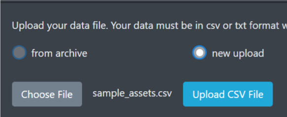
We temporarily save uploaded data files at archive.

Before next login, you don’t need to upload your data again.

Tick “from archive” and choose the file you have uploaded.

3.Configure simulation dates interval after uploading data.

(Note that: periodical rebalances begin from the first day of the interval.)

4.    Click “Next”.

2. Simulation Parameters

Next, you need to configure two important simulation parameters:

Data Window Size

Usually, rebalancing requires estimation of expectation and covariance of returns using historical data within a given period whose length is data window size. For example, If we set the window size to 6 months, when rebalancing on 1st July, 2010, the calculation will base merely on the data within 6 months(1st Jan. 2010 ~ 30th  Jun. 2010).

Rebalancing Period

This parameter is denoted by the interval between two adjacent rebalances.

You can configure more than 1 parameter sets.

Note that sometimes you may receive a warning like this:

This is because the data which will be used to do mean and covariance estimations for the first rebalancing are insufficient according to the window size. We need mean and covariance estimations based on the data in the window to rebalance.

If the data in the window are not enough, some errors will occur.

For example, if your file includes data from 2010-01-01 to 2019-01-01, your simulation start date is 2011-01-01 and data window size is 2 years, then the first rebalance will be based on 2009-01-01 to 2011-01-01. You don’t have the data from 2009-01-01 to 2009-12-31.

Possible solutions are:

1.Provide larger data file that includes earlier data;

2.Postpone your simulation start date;

3.Configure smaller data window size.

For example: if your source data starts on 2016-07-29 with a simulation start date 2016-10-29 and a 6 months data window size, methods to eliminate the warning for you will be:

1.Provide a data file that includes data beginning from 2016-04-29;

2.Set your simulation start date as 2017-01-29;

3.Set smaller data window size like 3 months or 1 month.

3. Portfolio-optimization Algorithms

Now you need to configure the portfolio-optimization algorithms for test.

We provide 4 kinds of algorithms: 1/N, Markowitz, SOCP and SAAM, where Markowitz, SOCP and SAAM are all based on modern portfolio theory.

1/N Algorithm

1/N represents equal weighting algorithm. At each rebalance, the whole money will be evenly distributed among all assets.

This algorithm is often used for comparison with other portfolio-optimization algorithms.

Markowitz Algorithm

Markowitz algorithm tries to balance benefits with risk based on investor’s risk aversion level. It solves

\(\max_{w} w^{T}r-\lambda w^{T} \Sigma w\) s.t. \(\ w^{T}1=1\)

SOCP Algorithm

Different from Markowitz’s quadratic programming solution, SOCP (second-order cone programming) is a convex optimization problem of the form

\(\min f^T x\)

subject to \(||{A_i x+b_i}||_2\) ≤ \(c_i^Tx+d_i\), i=1,2,…,m

\(F_x=g\)

where the problem parameters are f∈\(R^n\), \(A_i∈R^{d n_i*n}\), \(b_i∈R^{n_i}\), \(c_i∈R^n\)\(F∈R^{p*n}\), \(g∈R^p\).

\(x∈R^n\) is the optimization variable.

WHY SOCP?

When adding some complicated constraints into Markowitz model, the newly formed optimization problem may not belong to quadratic programming problems, so we introduce the more general programming method SOCP to solve the new problem. Solving a SOCP problem is also more time-efficient than solving the traditional quadratic programming problem even for original Markowitz model.

SAAM Algorithm

SAAM [1] (stochastic asset allocation method) develops Markowitz’s algorithm by considering future returns and risks as random variables. It solves

\(\max \limits_{η}\) {\(E[w^T(η)r_{n+1}]\)-\(\lambda Var[w^T(η)r_{n+1}]\)}

w(η)=arg \(\min \limits_{η}\) \(\lambda E[{w^Tr_{n+1}}^2]\)-\(ηE(w^Tr_{n+1})\)

SAAM also uses bootstrapping methods for resampling, which attenuates the bias of estimated effective weight vector.

More information about SAAM Algorithm can be seen here.

4. Algorithm Parameters

Parameters for each algorithm are as below:

For Markowitz and SOCP algorithms, we provide 3 methods to estimate returns.

Returns Estimation Models

Sample Mean:
Use mean of the sample data within the estimation window as returns.

\(r_i=\frac {\Sigma^m_{j=1}r_{ij}} {m}\)

Equal Mean:

Assume each asset shares the same expectation of return. Calculate average returns of all assets as each asset’s expectation of return.

\(\bar r\)=\(\frac {\Sigma^n_{i=1}r_i}{n}\)

Linear Shrinkage:

Based on Sample Mean but shrink to Equal Mean. The estimated expectation of return is calculated as below:

\(r_i^{′}\)=\((1-\sigma)r_i+\sigma\bar r\)

For SOCP and Markowitz algorithms, we provide 4 methods to estimate covariance matrix.

Covariance Matrix Estimation Models

Sample Covariance:

Use covariance of the sample data within the estimation window for estimation.

\(\Sigma=(\Sigma_{ij})\)

\(\Sigma_{ij}=\frac{1}{m-1}\Sigma_{k-1}^m (r_{ik}-r_i)(r_{jk}-r_j)\)

Equal correlation:

Assume every two different assets shares the same correlation, which is

\begin{equation}
\label{eq6}
\rho_{ij}=\left\{
\begin{aligned}
1, i=j; \\
c, i\ne j.
\end{aligned}
\right.
\end{equation}

where c is a constant.

Use maximum likelihood estimation to calculate this correlation and then the covariance matrix:

\(\Sigma_{ij}=Cov(X_i,X_j)=\rho_{ij}\sigma_i\sigma_j\)

Linear Shrinkage:

Based on Sample Covariance but shrink to Equal Correlation. The estimated expectation of covariance matrix is calculated as below:

\(\Sigma^{′}=(1-\delta)\Sigma+\delta F\)

        where F is the covariance matrix calculated by equal correlation method.

Nonlinear Shrinkage:

The best known method to estimate covariance matrix, introduced by Lediot and Wolf in this paper [2]

For SAAM algorithm, the following two parameters are available.

Returns Moments Estimator & Returns Resampling Model

These parameters are only for SAAM Algorithm. We now only provide Ledoit Wolf 2002 as returns moments estimator (this link) [3] and block bootstrap as returns resampling model.

Risk Aversion Coefficient

This is the λ in the model like Markowitz’s, like

\(\max \limits_w w^Tr-\lambda w^T\Sigma w\)

s.t. \(w^T1=1\)

Besides, we provide several constraint options for SOCP, Markowitz & SAAM.

*For Markowitz, its quadratic programming only enables you to configure Position Limits.

Constraints (Optional)

Market Impact:

Market impact describes the impact of investments to the market, which means, your investment weight vector w can influence expected return vector r.

We use non-linear model to depict this relationship, which is \(r_i^{′}=r_i-l_i \sqrt{w_i }\), where \(l_i\)s are square root impact coefficients. Larger it is, larger impact the corresponding asset has on the market.

To set square root impact coefficient for an asset,

tick the check box of the asset, fill in the number you want to set in the input box below, and click “Update”.

If you want to set the same coefficient for every asset, tick the check box

on the top left corner to select all, fill in the number in the box below and click “Update”.

You can set other constraints in the same way as the introduction in the last slide.

Position Limits:

Allowed minimum and maximum weight for any given assets.

  e.g. If you set minimum weight as 0, then short selling will not beallowed.

Black List:

Weights of black-listed assets will not be changed during transactions.

Max Loan:
This decides the minimal allowed weight of asset during transactions.

e.g. If you set max loan as 0.3, then the weight of asset can be at least -0.3.

Adding New Model

First, select a portfolio optimization algorithm.

If your algorithm is not 1/N,

then, choose the estimation models and click “add”;
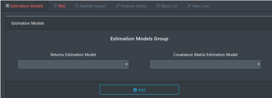
Then, click Risk tab and set risk aversion coefficient and constraints (introduced in former slides) .

Finally click “Finish the SOCP configuration”.

After finishing adding new models, click “Next” to configure diversification method.

5. Diversification

If you have chosen Markowitz, SOCP or SAAM method before, you will be able to choose whether to use Corvalan algorithm to do some diversification.

Corvalan Algorithm

Corvalan method adds a tolerance term in strict equalities of the original model.

Suppose the optimal solution of the original problem is w, the corresponding expected return is \(R=w^Tr\), and variance is \(\sigma=w^T\Sigma w\). Then Corvalan method solves the model below:

\(\min\limits_{v}f(v)\)

s.t. \(v^Tr\geq R(1-\Delta r)\), \(v^T\Sigma_v\leq\sigma (1-\Delta\sigma)\) and other constraints

where f(v) is a function that will be very large if v fails to be well-diversified.

This algorithm solves the problem that the weight vector calculated by Markowitz-like models often concentrate on only several assets.

To add diversification model, just select Corvalan algorithm and set Relaxation of Expected Returns

Δr(%) and Relaxation of Covariance Δσ(%) and click “Next”. They are parameters in the model below:

\(\min\limits_{v}f(v)\)

s.t. \(v^Tr\geq R(1-\Delta r)\), \(v^T\Sigma_v\leq\sigma (1-\Delta\sigma)\) and other constraints

6. Run & Check

After configuring models, we go to the page “configurations of models”.

Tick the configurations you would like to simulate and click “Run the Selected Configurations”.

After simulations accomplish, the system would send you a prompt.

Click “Reports” on the left to check the results.


In this page, you can either check the results separately, or check them together and compare.

If you just want to check one result, click its Configuration Name.

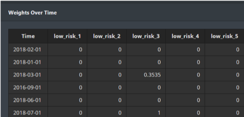
Reports include profit & loss plot, vital performance measures, weight over time and executions.

You can download report including details.

We also provide .csv format file (executions, measures, weights) for you to download and analyze.

To compare several models, tick them all and click “Simulation Comparison”.

The system will plot their profit & loss on the same canvas, and provide the comparison of vital performance measures.

Performance Measures

We provide 32 measures on the webpage to help you to analyze whether your model performances well.

For example

Cumulative Return;
Commission;
Max. Drawdown%:

The worst (the maximum) peak to valley loss since the investment’s inception.

Execution Count:

The number of sell/buy orders you have made.

Treynor ratio:

The risk premium obtained per unit of risk. The greater the Treynor index, the higher the unit risk premium is and the better the performance of the portfolio is. Calculation follows below:

\(TR=\frac{R_p-R_f}{\beta_p}\)

These measures could all be found in measures.csv . You can download it and see more detailed analysis.

Simulation of mean-reverting portfolio computed by daspremont2008 model

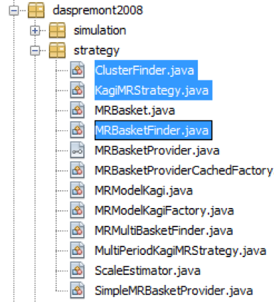
  1. Open MultiPeriodKagiMRStrategyDemo.java
  2. The simulation parameters are defined in the class MRSimParamSP500.
  3. Open MRSimParamSP500.java
  4. MRSimParamSP500 defines the pool of stocks in which the mean-reverting baskets of stocks will be found. Also, it defines the number of baskets, the size of each basket, the time interval of the simulation, how frequent the basket is renewed, how far historical price data is used for computing the optimal clusters and baskets, etc.
  5. Run the simulation. Right-click “MultiPeriodKagiMRStrategyDemo.java” and select “Run File”.
  6. It starts by downloading the price data from Yahoo server to the hard drive.
  7. Then, it finds clusters of related stocks based on covariance selection (matrix optimization with penalty). Please see “com.numericalmethod.algoquant.model.daspremont2008.strategy.ClusterFinder” for details.
  8. Within the largest cluster(s), mean-reverting baskets are found (using SDP). Please see “com.numericalmethod.algoquant.model.daspremont2008.strategy.MRBasketFinder” for details.
  9. The mean-reverting baskets are traded with KAGI strategy. The output will show the simulation results. Please see “com.numericalmethod.algoquant.model.daspremont2008.strategy.KagiMRStrategy” for details.
  10. The computed baskets and their price series are saved as CSV files in the “log” folder for reference.


Besides, users can also choose other mean-reverting strategies in AlgoQuant to trade the mean-reverting baskets:

com.numericalmethod.algoquant.model.elliott2005

com.numericalmethod.algoquant.model.jurek2007

com.numericalmethod.algoquant.model.volarb


Utility Formula

By introducing the concept of risk and efficient frontier, Markowitz inaugurated a sort of modern securities portfolio management.

In a portfolio of securities whose returns and volatility are known, and in which the price movement of one does not completely influence that of the other, it is possible to calculate the weight of each security in order to achieve maximum performance while taking the minimum risk. From an objective and rational perspective, investors should always choose the optimal portfolio with the minimum risk relative to the chosen level of returns.

But what is the level of risk the investor is able to endure? The answer is subjective. This is how the utility formula and risk aversion coefficient introduce to portfolio management.

  • Risk Aversion Coefficient

A quantitative and practical method will be used to measure the risk aversion of an investor. The risk aversion coefficient can be considered as what an investor is willing to sacrifice expected return in order to lower variance by one unit. A higher risk aversion coefficient means investor are more willingly to pass up the opportunity for a large gain in favor of safety. Since it is a trade-off between risk and return, the risk aversion coefficient has to be positive for the portfolio optimization.

  • Mean-Variance(quadratic) Utility Formula:

\(U = \mathop{\mathbb{E}[R]} – 0.5 \ast A\ast {\sigma}^2 \)

In this formula, U represents the utility or score to give this investment in a given portfolio by comparing it to a risk-free investment.
\(\mathop{\mathbb{E}[R]} \) is the expected return of the portfolio and \({\sigma}^2 \) is the square of volatility.
The part of the equation to the right of the “minus” sign indicates the risk of the strategy itself, taking into account the investor’s risk aversion. The formula as a whole therefore gives us the difference between the total expected return of a portfolio and the risk involved.

Well Diversified Efficient Portfolios

Well Diversified Efficient Portfolios

Investors scarcely use mean-variance optimization when deciding on their actual portfolios. One of the main reasons they give is that efficient portfolios are systematically concentrated in a few assets. This article shows that such an allocation is achieved when portfolio risk and return are seen as infinitely accurate magnitudes. However, if the frontier is considered within some infinitesimal tolerance, as in a one-hundredth neighborhood, there are thousands of efficient portfolios and, indeed, many of them are well diversified.

Download

NMRMS User Guide

Step 1: Portfolio Construction

There are two ways to construction user’s portfolio. Users can upload their portfolio file or construct their portfolio with our stock database.

1.1 Upload Own Data

Users can optimize any portfolio that they upload online.

  1. New upload: upload a new portfolio dataset.
  2. From archive: choose pre-uploaded and temporarily saved portfolio data.

Tips:

The filename extension should be (.csv) or (.txt) with ‘,’ as separator.
The first row should be names of assets.
The first column should be a date sequence.
Each cell represents the price of an asset at a certain date.
An example of portfolio file can be downloaded as sample data.
Note that the start date and end date must be within the original dataset.

  1. Set Data Window Size
    The data window size indicates the length of historical data used for estimating  assets’ return and covariance. Please make sure the data window is at least 4 times the rebalancing period. 
  2. Set Rebalancing Period
    This parameter is denoted by the interval between two adjacent rebalances, which is the process of realigning the weightings of a portfolio of assets to maintain an original or desired level of asset allocation or risk. The shorter the rebalancing period, the more frequent the portfolio will be set to its optimal weights based on optimization algorithm.
  3. Click ‘Add’
    User can add multi/different parameter sets for the simulation, optimization and comparison.
  4. Click “Next”

1.2 Load from Database

User can construct the portfolio with our equity database.

1. First user need to set the start date and end date as the back testing period. And the data window size and rebalancing period for the portfolio construction.

2.In the stock selection page, we provide two methods to add stocks to user’s portfolio. The simplest method is searching stock by its ticker*.
*User can add stocks to white list by searching their tickers or companys’ name. All the stocks in white list will be added to portfolio even if they don’t fit the filters.And we have filters for user who have specific idea of the kinds of stocks which meet their standards and suit their strategies. For examples:

  • Use ‘market cap’ to find large cap or small cap stocks
  • Use ‘sector’ to find stocks in a particular industry
  • Use ‘P/E (price-to-earning ratio)’ to select value or growth stocks

Multiple filters can be applied to help the user to find the stocks for their portfolio, and we also provide an easy way to delete all the applied filters all at once.

Notice some filters provide both ‘Percentile’ filter and ‘Min/Max’ filter to fit different needs. User can change it by clicking the filter name.

3.Stocks that have been selected by filters will show in the table below. And all these stocks will be added to user’s portfolio.
Notice selected stocks will be automatically propagate to the portfolios of following rebalancing dates, which means the portfolio will not change in the following rebalancing dates even if some of the stocks are not fit the filters.Step 2: Add portfolio-optimization algorithms

Step 2: Choose optimization model

In this part, we introduce 4 kinds of algorithms and correspondingly parameters first, and then we have a brief view towards other constraints.

1) 1/N algorithm

No parameter for this algorithm

2) Markowitz algorithm

  1. Choose Returns Estimation Model from the following 3 methods: sample mean, equal mean and linear shrinkage (with Shrinkage Parameter δ).
  2. Choose Covariance Matrix Estimation Model from the following 4 methods: sample covariance, equal correlation, linear shrinkage (with Shrinkage Parameter δ) and nonlinear
    shrinkage.
  3. Input Risk Aversion Coefficient with positive value.
  4. Set Position Limits with min and max value for selected asset (optional)

3) SOCP algorithm

  1. Choose Returns Estimation Model from the following 3 methods: sample mean, equal mean and linear shrinkage (with Shrinkage Parameter δ).
  2. Choose Covariance Matrix Estimation Model from the following 4 methods: sample covariance, equal correlation, linear shrinkage (with Shrinkage Parameter δ) and nonlinear shrinkage.
  3. Input Risk Aversion Coefficient with positive value.
  4. Set Market Impact with Square Root Impact Coefficient for selected asset (optional).
  5. Set Position Limits with min and max value for selected asset (optional).
  6. Choose Block List (optional).
  7. Set Max Loan for selected asset (optional).

4) SAAM algorithm

  1. Choose Returns Estimation Model with method Ledoit Wolf 2002
  2. Choose Portfolio Returns Resampling Model with method block boostrap
  3. Input Risk Aversion Coefficient with positive value.
  4. Set Market Impact with Square Root Impact Coefficient for selected asset
    (optional).
  5. Set Position Limits with min and max value for selected asset (optional).
  6. Choose Block List (optional).
  7. Set Max Loan for selected asset (optional).

※To set square root impact coefficient for an asset, tick the check box of the asset, fill in the number you want to set in the input box below, and click “Update”. Other optional constraints can be set similarly.

※If you want to set the same coefficient for every asset, tick the check box on the top left corner to select all, fill in the number in the box below and click “Update”. Other optional constraints can be set similarly.

Step 3: Configure diversification method and corresponding parameters (optional)

With optimization methods of Markowitz, SOCP or SAAM algorithm, users can choose Corvalan
algorithm for portfolio diversification.

  1. Set Relaxation of Expected Returns Δr
  2. Set Relaxation of Covariance Δσ

For more details, see :  Diversification Method

Step4: Run simulations and view outputs

  1. Select the newly-added model under the data source
  2. Click ‘To do’
  3. Run stimulations
  4. Report

Corporate Investment Factors

Capital Expense to Sales Ratio

CAPEX to Sales Ratio measures the level of investments a company is making into its future. CAPEX value will be positive for expenditures.
CAPEX to Sales Ratio = (CAPEX in quarter t / Net Sales in quarter t)
CAPEX to Sales Ratio TTM = (CAPEX ttm / Net Sales TTM)
Net sales MUST be POSITIVE

Capital Expense to Total Assets Ratio

CAPEX to Assets Ratio compares the level of investments a company is making with its assets. CAPEX value will be positive for expenditures.
CAPEX to Assets Ratio = (CAPEX in quarter t / Assets in quarter t)
CAPEX to Assets Ratio TTM= (CAPEX TTM / Assets TTM)
Assets MUST be POSITIVE

Investment Growth Ratio

Investment growth is the growth rate in capital expenditure. Firm capital investment, determined by Tobin’s Q, which is proxied by firms’ market-to-book ratios, relates to future equity returns in the same way as the market-to-book ratio.  CAPEX value will be positive for expenditures.
Investment Yearly Growth Ratio (ig_yoy) = (CAPEX in quarter t / CAPEX in quarter t – 4)
Investment Quarterly Growth Ratio (ig_qoq) = (CAPEX in quarter t / CAPEX in quarter t – 1)

Assets Growth Ratio

Assets growth ratio measures the degree to company’s asset increases or decreases in value over time.
Assets Yearly Growth Ratio (ia_yoy) = (Assets in quarter t / Assets in quarter t – 4)
Assets Quarterly Growth Ratio (ia_qoq) = (Assets in quarter t / Assets in quarter t – 1)

Inventory Growth Ratio

Inventory investment is highly correlated with the business cycle. Inventory growth ratio, measures as the increase or decrease in firm’s inventory over a year, represents a firm’s productivity and it’s business cycle.
Inventory Yearly Growth Ratio (ivg_yoy) = (Inventory in quarter t / Inventory in quarter t – 4)
Inventory Quarterly Growth Ratio (ivg_qoq) = (Inventory in quarter t / Inventory in quarter t – 1)

Quick Ratio

Quick ratio is an indicator of a company’s short-term liquidity position and measures a company’s ability to meet its short-term obligations with its most liquid assets.
quick_ratio = (current assets – inventory)/current liabilities *100
Current liabilities MUST be POSITIVE

Current Ratio

Current ratio is a liquidity ratio that measures a company’s ability to pay short-term obligations or those due within one year with its current assets.
current_ratio = current assets / current liabilities *100
Current liabilities MUST be POSITIVE

Inventories Changes to Assets Ratio

Inventory changes is the change in inventory of quarter t scaled by the average of total assets of quarter t and t-1
Inventory changes to Assets Ratio = (inventory in quarter t – inventory in quarter t-1)/((assets in quarter t + assets in quarter t-1)/2)*100;
assets MUST be POSITIVE.

Inventories to Current Assets Ratio

Inventories to Current Assets Ratio measures the portion of current assets tied up in inventory.
Inventories to Current Assets Ratio = inventory / Current assets * 100;
Inventories to Current Assets Ratio TTM = inventory 12 month average / Current assets *100
Current assets MUST be POSITIVE.

Changes in PPE and Inventories to Assets Ratio

Changes in PPE and Inventories to Assets Ratio is defined as the annual change in gross property, plant, and equipment plus the annual change in inventory scaled by one-year-lagged total assets.
Changes in PPE and Inventories to Assets Ratio = ((inventory in quarter t – inventory in quarter t-4) + (PP&E in quarter t – PP&E in quarter t-4)) / assets in quarter t-4 * 100
Assets MUST be POSITIVE.

Net Operating Assets to Assets Ratio

Net Operating Assets to Assets Ratio is net operating assets scalded by one-year-lagged total assets. Net operating assets measures as operating assets minus operating liabilities.
Net Operating Assets to Assets Ratio = (operating assets – operating liabilities)/assets*100
Net Operating Assets to Assets Ratio TTM = (operating assets TTM – operating liabilities TTM )/assets*100
Assets MUST be POSITIVE.

Changes in Net Operating Assets to Assets Ratio

Changes in net operating assets, dNoa, is the quarterly change in net operating assets scaled by lagged total assets.
Changes in Net Operating Assets to Assets Ratio = (noa in quarter t – noa in quarter t -1)/assets in quarter t-1 *100
Assets MUST be POSITIVE.

Changes in long-term Net Operating Assets to Assets Ratio

Changes in long-term net operating assets measures as the change in net PP&E plus the change in intangibles plus the change in other long-term assets minus the change in other long-term liabilities and plus depreciation and amortization expense. d_lt_noa_assets is the change in long-term net operating assets scaled by the average of total assets from the current and prior quarter.
long-term net operating assets (lt_noa) = intangibles + long-term assets + long-term liabilities – long-term debt
change in long-term net operating assets (d_lt_noa) = lt_noa in quarter t – lt_noa in quarter t-1 + depreciation expense
Changes in long-term Net Operating Assets to Assets Ratio (d_lt_noa_assets) = d_lt_noa / ((assets in quarter t + assets in quarter t-1)/2)*100
Changes in long-term Net Operating Assets to Assets Ratio TTM = d_lt_noa TTM / ((assets in quarter t + assets in quarter t-1)/2)*100
Assets MUST be POSITIVE.

Operating Accruals to Assets Ratio

Operating Accruals measures as the statement of cash flows as net income (item NI) minus net cash flow from operations. Operating accruals to assets ratio (Oa_assets) calculated by Operating Accruals scaled by total assets.
Operating Accruals to Assets Ratio (oa_assets) = (net income – operating net cash flow) / assets*100
Operating Accruals to Assets Ratio TTM (oa_assets_ttm) = (net income – operating activities net cash flow) 12 month average /assets*100
Assets MUST be POSITIVE.

Total Accruals to Assets Ratio

We use the cash flow approach to measure Total Accruals as net income minus total operating, investing, and financing cash flows plus sales of stocks minus stock repurchases and dividends. Total accruals to assets ratio (Ta_assets) is calculated as Total Accruals scaled by total assets.
total accruals = net income – operating net cash flow – investing net cash flow – financing net cash flow + stock repurchase + cash dividends
Total Accruals to Assets Ratio (ta_assets) = total accruals / assets *100
Total Accruals to Assets Ratio TTM (ta_assets_ttm) = total accruals 12 month average / assets *100
Assets MUST be POSITIVE.

Percent Operating Accruals

Percent Operating Accruals scaled operating accruals by the absolute value of earnings as percent accruals.
Percent Operating Accruals (perc_oa) = (net income – operating net cash flow) / abs(net income) *100
Percent Operating Accruals TTM (perc_oa_ttm) = (net income – operating net cash flow) 12 month average / abs(net income 12 month average) *100

Percent Total Accruals

Percent Total Accruals calculated as total accruals scaled by the absolute value of net income.
Percent Total Accruals (perc_ta) = total accruals / abs(net income)*100
Percent Total Accruals TTM (perc_ta_ttm) = total accruals 12 month average / abs(net income 12 month average)*100