PolyModel and Risk Management
- Replace one function\(Y=f(X_1,…,X_n)+\epsilon\)
by a collection:
\(Y=f_1(X_1)+\epsilon_1\) \(f_1(X_1)=E[Y|X_1]\)
…
\(Y=f_n(X_n)+\epsilon_n\) \(f_n(X_n)=E[Y|X_n]\)
Taken individually, each model is imprecise, but the collection contains much more information than a multi-factor model!
- Individual models can be nonlinear and contain lags
- Easy to calibrate
- Focus on where useful info lies: in the extremes
- Factors can be correlated and linearly, or even nonlinearly dependent
- Use hundreds, or even thousands of factors
- Need to assess the relevance of each factor ⇒Score =-Ln(p-value)
By definition, a “model” is aimed at stressing a fund or an asset and anticipate its response to the stress
A PolyModel is a Collection of Single-Factor (Nonlinear) Models
- Step 1: Identify a LARGE Set of Factors
- LONG HISTORY (20+ Yrs incl. crises)
- As many factors as potential risk sources ⇒Several 100’s
- Step 2: Scan Factors One at a Time
- Focus on EXTREME MOVES⇒Nonlinear Models
- Select only factors with a strong statistical relationship to the fund Þ Score = –Ln(p-value)
- A risk factor is selected if its Score is at least ½ highest score across all factors
- Step 3: Stress Selected Factors
- 99%-Confidence Worst Impact of each Selected Factor
- Single Factor \(StressVAR=√(Worst Impact)^2+(Specific Risk)^2\)
- Global STRESS VaR = MAX(Single Factor Stress VaR)
- Handle 100’s of Market Factors
- Model rare events (“Black Swans”)
- More accurate when needed, than when not needed!
- Tail concentration effect
- Suited for risk measurement and stress scenarios
- Prediction from individual factors can be merged
- Risk measure = STRESS VaR (worst case) includes hidden risks
- Can be aggregated for a portfolio
- Risk contributions involve extreme correlations
- Superior allocation and optimization
- Risk Factor: X(t)
- Invested Asset: Y(t)
- Bayesian Computation of E(Y|X)
- Prior regime probabilities: ergodic limit \(\pi_k\)(uninformed Jeffreys prior)
- Given the value of X, compute the implied (posterior) probabilities
\(p_k(X)\)
\(E_{R_k}(Y|X)=a_kX+b_k\) linear for one regime
\(E(Y|X)=\Sigma^m_{k=1}p_k(X)E_{R_k}(Y|X)=f(X)\) with nonlinear f in multi-regimes
- The more probabilities are sensitive to X, the more nonlinear is f ⇒PolyModels used as Crisis indicator
- HMM is a dynamic model that can be simulated
- PolyModels are a statistical analysis of the dynamics
Question: Fund risks and future returns?
Input: PolyModel (instead of series of returns)
- Uses market information⇒Sensitivity to risk factors
Answer:
- Selects funds that have a convex (antifragile) response to dominant factors
- Rejects funds that have a concave (fragile) response to dominant factors
Advanced methods (to be tested)
- Deep learning
- Adversarial learning
Learning to “guess the future”: contradicts Market Efficiency Hypothesis
Learning risks with behavior under stress: Use sensitivity to factors as input
Unsupervised Learning
- Train the system on all past situations to predict returns
⇒Efficient Market Hypothesis!!!
- No expected return, most likely lured by Black Swan risk
- Predict volatility (or another risk measure): possible, but doesn’t produce a trading signal
Supervised Learning
- Build a Risk Profile for each asset: list of responses to stress tests
- Train the allocation system (across asset classes and within each asset class) on the basis of the Risk profile
- Performance, volatility are not predicting future regime change
- Downturn Indicator: Left skew, fragility
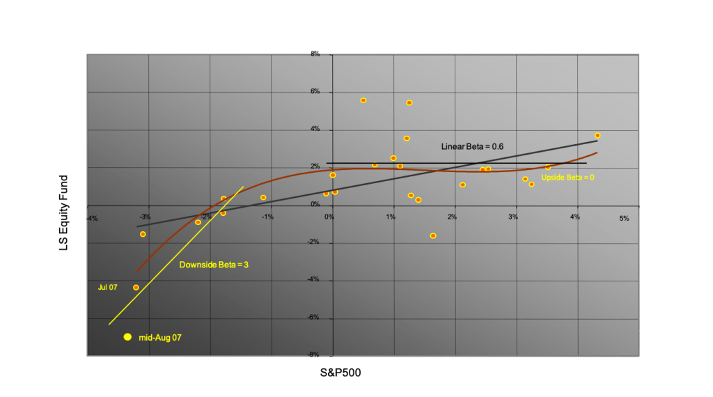
Long-Short Equity Fund Beta change in a systematic manner
The traditional linear Beta of the fund is 0.6.
But by carefully examining these returns, one finds that the “upside Beta” is 0, while the “downside Beta” reaches 3.
Had the S&P fallen by 15% instead of 5%, the fund would have lost an extra 30%, reaching almost 40%, sufficient to put it out of business.


