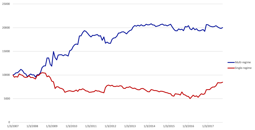
Multi-Regime Portfolio Optimization
Overview
- Identification of Current Regime
- MCMC simulated over a given period of time (e.g. one month)
- Expected Return of each asset
- Monte-Carlo simulation⇒VaR of any virtual portfolio (Gaussian mixture)
- Maximization of Expected Return / VaR
- Rebalancing based on dynamic criterion (profit taking) and/or signal strength
- Benchmark: Same with 1 regime = Markowitz
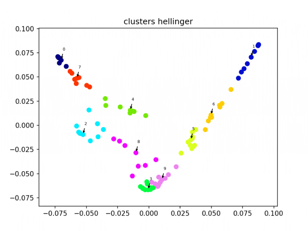
Spectral Embedding and Clustering
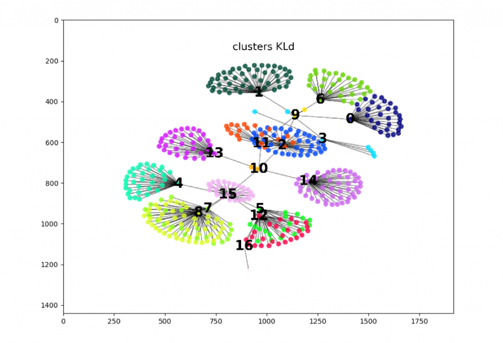
Clustering by Tree Algorithm
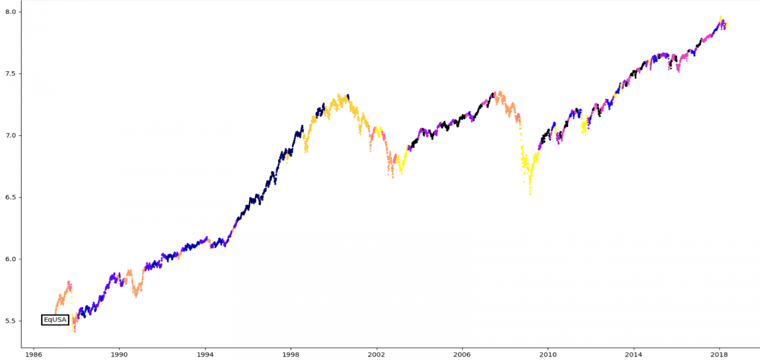
Regime Sequence
- Assume that Y1…Ym have mixed joint distribution
\(\ P = \pi_1P_1+…+\pi_qP_q\) with \(\pi_1>…>\pi_q\)
- Fat tails can be measured as the ratio of risk under P1 risk under other regimes.
- An optimizer that only accounts for some regimes will reduce the risk under those regimes, but increase the risk under other regimes, hence increasing fat-tailedness
⇒Regime changes have an aggravated impact on portfolio risk
Dynamics in the Market Variable Space
- Finite Number of Regimes R1,…,Rm
- Covariance Matrix Gk
- Drift Vector mk
- Rk ~ N(mk,Gk)
- Transition Probability Matrix
- P(t,t+1) = (phk)
- phk = Probability of transitioning from Rh to Rk
- ∀h, \(\Sigma^m_{k=1}p_{hk}=1\)
- P(t,t+n) = Pn
- Euler Scheme:
- Discretized Time t0,…,tn
- Pick new regime R(ti+1) according to P applied to current regime R(ti)
- Simulate Market Evolution following R(ti+1)
- Gaussian Mixture ⇒ “Fat Tails”
- Asymptotically Gaussian
- \(\mu_∞=\Sigma^m_{k=1}\pi_k\mu_k\)
- \(\Gamma_∞=\Sigma^m_{k=1}\pi_k\Gamma_k\)
- P’ \(\pi=\pi\), \(\pi=(\pi_1,…,\pi_m)\)
- Determine Breakpoints(\({t_1,…,t_n}\)) and “homogenous” periods \(J_k=[t_{k-1},t_k]\)
- Calibrate a Gaussian distribution\(N(\mu_k,\Gamma_k)\) over consecutive periods \(J_k\)
- Clusterize the set of \(\Phi=(\mu_k,\Gamma_k)\), using some information distance (K-L, Tsallis, Hellinger…)
- Issue: these distributions lie in a high dimensional space n(n + 3)/2⇒No recurrence
- Reduce dimension by describing the market with fewer indices
- Project \(\Phi_k\) onto a lower dimensional space, approximately preserving distances, using Spectral Embedding
- Common practice: focus only on volatility
- The projection now has some recurrence.
- Estimate Transition Probabilities
- Baum-Welch algorithm: too imprecise
- SVM or EM provide more accurate results
- Depends on time spent within a regime
- Crisis Prediction: Mild regime that is likely to transit to a wild one
Multi-Regime Simulation vs. Observed
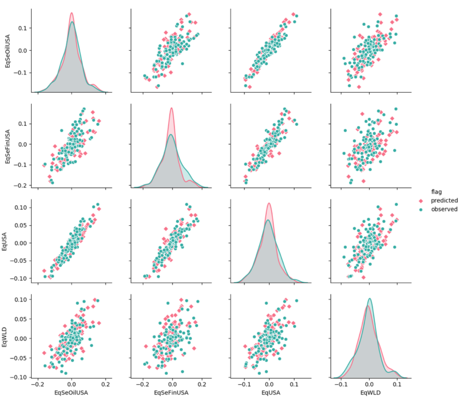
Pink: Multi-Guassian Simulation (MCMC)
Green: Actual Returns
Joint distribution of 4 risk factors:
SP500
SP Sector Financials
SP Sector Oil Companies
MSCI World
Simulation on US Market
