Markowitz’s mean-variance model & Application in NM System
Harry Markowitz pioneered the Markowitz model in his paper “Portfolio Selection,” which was published in the Journal of Finance in 1952, and was recognized by the Nobel Prize committee in 1990. This model explains how risk-averse investors use portfolio investment to create more alternative investment opportunities, in order to obtain the maximum expected rate of return under a certain risk or to minimize the investment risk under a certain expected rate of return.
Markowitz’s mean-variance model extracts two important characteristics of the assets’ return rate-the expected return rate and the variance of the return rate. Markowitz defines the investment risk as the variance of the rate of return and assumes that people’s investment principle is to obtain the highest possible rate of return with the smallest possible variance (risk). The model calculates the effective boundary of the investment portfolio based on the expected return rate, the variance of each security, and the covariance matrix between the asset return rate. Given an indifference curve that reflects investor preferences, we will be able to obtain the optimal ratio of investment in each asset.
Examples:
Assume that investors can choose between asset A and B. The expected return rate, standard deviation, and correlation of assets are shown in the following table:
|
A |
B |
|
|
E(r) |
20% |
15% |
|
Standard deviation |
28.70% |
20.50% |
|
covariance |
0.023 |
|
|
correlation |
0.390924 |
|
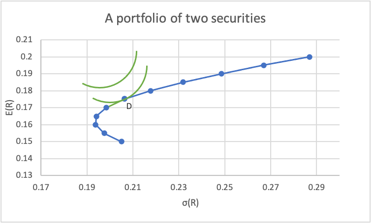
Investors invest all their funds in a certain combination of A and B. The following table shows the expected return and standard deviation of the portfolio under different combinations of A and B.
|
A |
B |
E |
sd |
|
0 |
1 |
0.15 |
0.205 |
|
0.1 |
0.9 |
0.155 |
0.197494 |
|
0.2 |
0.8 |
0.16 |
0.19378 |
|
0.3 |
0.7 |
0.165 |
0.194076 |
|
0.4 |
0.6 |
0.17 |
0.198363 |
|
0.5 |
0.5 |
0.175 |
0.206394 |
|
0.6 |
0.4 |
0.18 |
0.217754 |
|
0.7 |
0.3 |
0.185 |
0.231955 |
|
0.8 |
0.2 |
0.19 |
0.24851 |
|
0.9 |
0.1 |
0.195 |
0.266982 |
|
1 |
0 |
0.2 |
0.287 |
Through calculation, we get the expected return rate and variance curve of the investment portfolio of the two assets. At the turning point of the curve, we can find the minimum variance portfolio. At the upper part of this point, as the return on the portfolio increases, its variance(risk) also increases.
The curve is tangent to the indifference curve of a given investor at point D. The investment portfolio at point D for this investor is the best investment portfolio.
Disadvantage
The investment ratio estimated by Markowitz’s mean-variance model is sensitive to one of the core inputs of the model, which is the expected return. When the expected return on assets slightly changes, the investment portfolio ratio may change significantly. The robustness of the model is insufficient. Moreover, the expected rate of return is the prediction of the future, which is usually difficult to estimate accurately.
Use Markowitz in NM system:
- Choose Returns Estimation Model from the following 3 methods: sample mean, equal mean and linear shrinkage (with Shrinkage Parameter δ).

- Sample mean : Use mean of the sample data in the estimation window as expected returns
- Linear shrinkage: Pulling the extreme mean values toward the portfolio average.
- Equal mean: Assume each asset has the same expected return. This essentially ignores the portfolio return maximizing part. It gives a minimum variance portfolio, one of the smart beta portfolios.
2. Choose Covariance Matrix Estimation Model from the following 4 methods: sample covariance, equal correlation, linear shrinkage (with Shrinkage Parameter δ) and nonlinear shrinkage.
- Sample covariance: Use the sample covariance of the data within the estimation window.
- Equal correlation: Assume every two different assets has the same correlation.
- Linear shrinkage: Pull the extreme covariance values toward the group mean.
- Nonlinear shrinkage:Individually modify the extreme covariance values. This is the best known method to estimate covariance matrix.
- Input Risk Aversion Coefficient with positive value.
- “Risk Aversion Coefficient”: A higher risk aversion coefficient means investor are more willingly to aim for higher portfolio return by risking a more risky or volatile portfolio
4. Set Position Limits with min and max value for selected asset (optional)
- You can use “Position Limits” to set minimum and maximum weight for any assets. For example, if you set all minimum weight to 0, then short selling will not be allowed, hence a long-only portfolio


