// PM // Risk management

PolyModel

Replace one multi-factor regression with a collection of single-factor, nonlinear models. Each model alone is imprecise, but together they hold far more information than a multi-factor model — and they reveal how a fund or asset behaves under stress.

// Principle

One function becomes a collection

Instead of

Y = f(X₁, …, Xₙ) + ε

use

Y = f₁(X₁) + ε₁, f₁(X₁) = E[Y | X₁]

…

Y = fₙ(Xₙ) + εₙ, fₙ(Xₙ) = E[Y | Xₙ]

›Individual models can be nonlinear and include lags — easy to calibrate, and focused where the useful information lies: the extremes.
›Factors may be correlated, even nonlinearly dependent, so hundreds or thousands of them can be used at once.
›Each factor's relevance is scored as Score = −ln(p-value).

// Method

Three steps to Stress VaR

STEP 1

Identify a large set of factors

›Long history: 20+ years including crises
›One factor per potential risk source — several hundred

STEP 2

Scan factors one at a time

›Focus on extreme moves with nonlinear models
›Keep only factors with a strong statistical link to the fund
›Select a factor if its score is at least half the highest score

STEP 3

Stress the selected factors

›99%-confidence worst impact of each selected factor
›Single-factor Stress VaR = √(worst impact² + specific risk²)
›Global Stress VaR = max of single-factor Stress VaRs

// Benefits

Risk measurement by PolyModels

›Handles hundreds of market factors
›Models rare events (“black swans”)
›More accurate when it matters — the tail-concentration effect
›Suited to both risk measurement and stress scenarios; Stress VaR captures hidden risks
›Aggregates across a portfolio: risk contributions use extreme correlations for better allocation and optimization

// Regimes

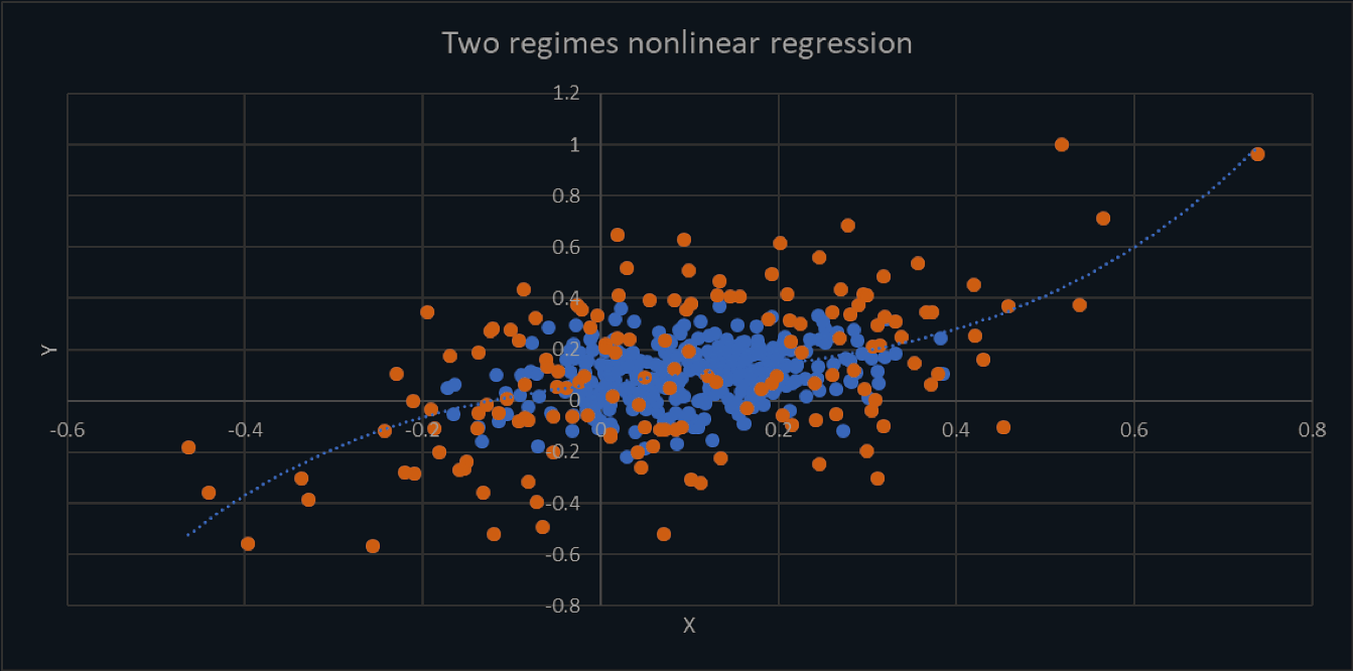
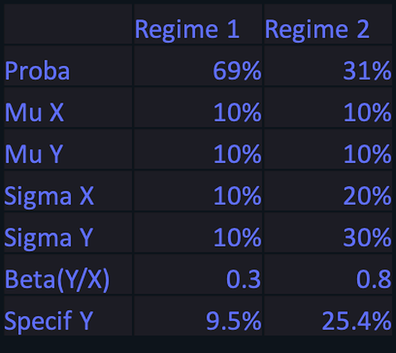
PolyModels in a hidden Markov model

›Risk factor X(t), invested asset Y(t); E(Y|X) computed in a Bayesian way.
›Prior regime probabilities are the ergodic limit πₖ; given X, compute posterior probabilities pₖ(X).
›Within one regime the response is linear: E_Rₖ(Y|X) = aₖX + bₖ.
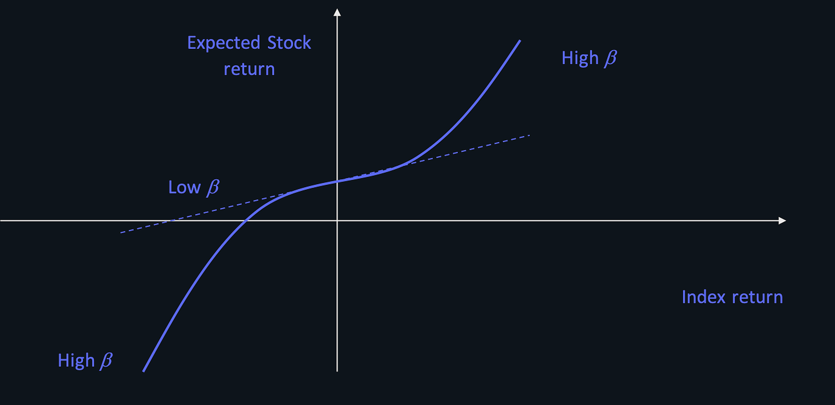
›Across regimes, E(Y|X) = Σ pₖ(X)·E_Rₖ(Y|X) = f(X) is nonlinear — the more the probabilities react to X, the more nonlinear f becomes, making PolyModels a crisis indicator.
›The HMM is a dynamic model that can be simulated; PolyModels are the statistical analysis of its dynamics.

// Machine learning

Learning risk, not guessing the future

Unsupervised

Training on past returns to predict returns runs into market efficiency: no reliable expected return, and a strong pull towards hidden black-swan risk. Predicting volatility is possible but yields no trading signal.

Supervised (PolyModel input)

Build a risk profile for each asset — its responses to stress tests — and train the allocation system on that profile. Funds with a convex (antifragile) response to dominant factors are selected; funds with a concave (fragile) response are rejected. Left skew and fragility act as downturn indicators. Deep and adversarial learning are being evaluated.

// Case study

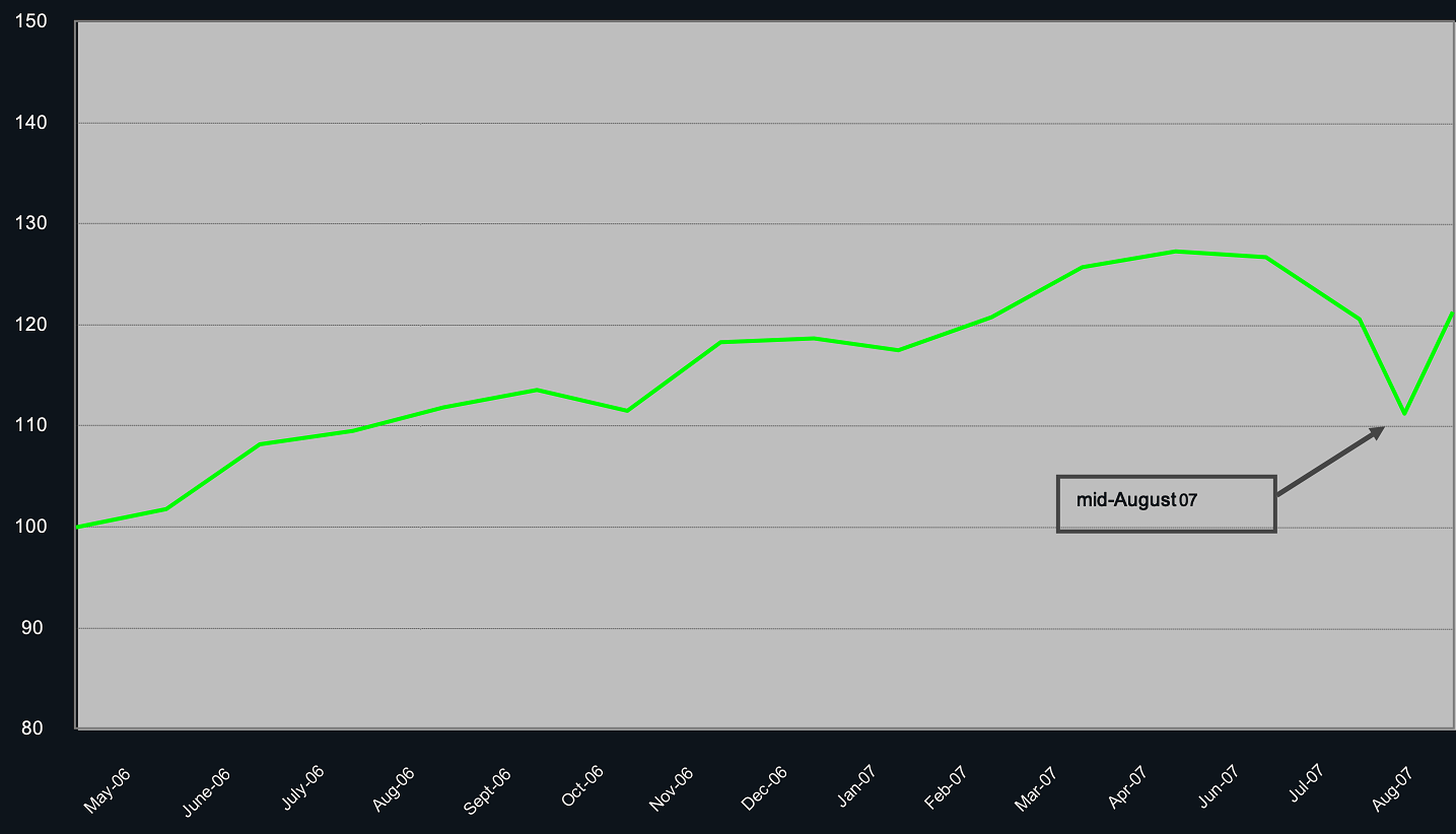
A long-short equity hedge fund

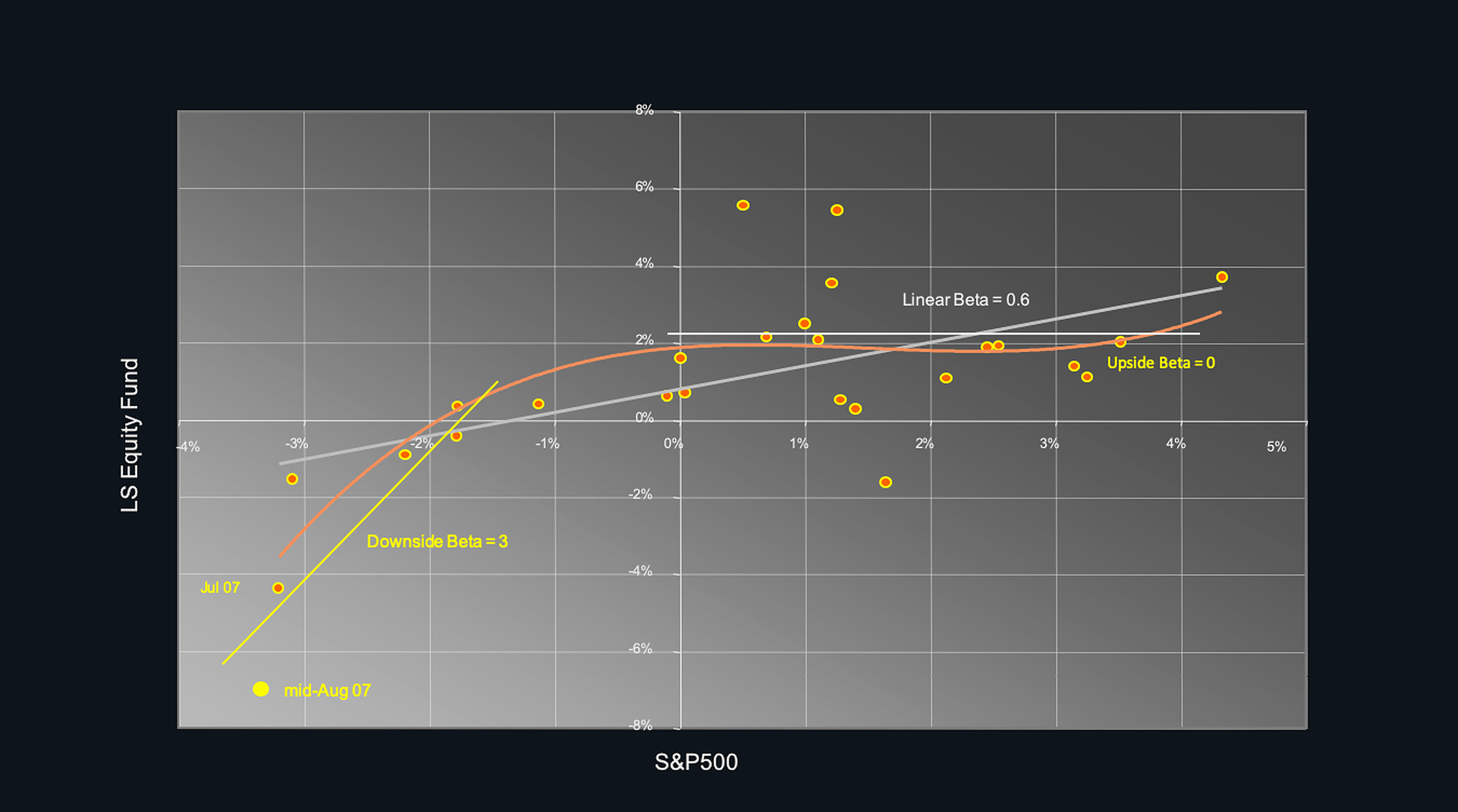
›A long-short equity hedge fund showed a traditional linear beta of 0.6 to the S&P 500.
›Its beta changed systematically: the upside beta was 0, while the downside beta reached 3.
›Had the S&P fallen 15% instead of 5%, the fund would have lost an extra 30% — almost 40% in total, enough to put it out of business.

Long-short equity fund NAV, May 2006 – Aug 2007

Talk to us about PolyModel →