// MR // Portfolio optimization

Multi-Regime Portfolio Optimization

Markets move between regimes — calm, stressed, crisis — each with its own drifts and correlations. Multi-Regime Portfolio Optimization identifies the current regime, simulates the market forward through regime transitions, and builds portfolios that stay robust when the regime changes.

// Overview

How it works

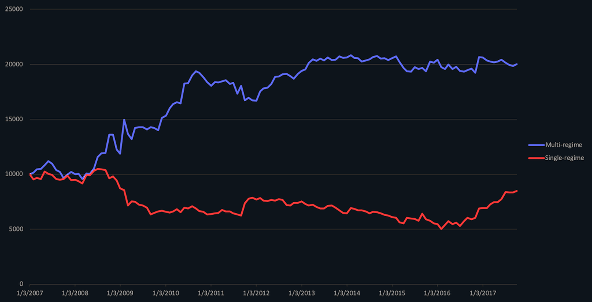
01Identify the current market regime.
02Run a Markov Chain Monte-Carlo simulation over a horizon (e.g. one month) to obtain each asset's expected return and the VaR of any portfolio under a Gaussian mixture.
03Maximize expected return / VaR.
04Rebalance on a dynamic criterion (profit taking) and/or signal strength.
05Benchmark: the same model with one regime, i.e. Markowitz.

// Regime identification

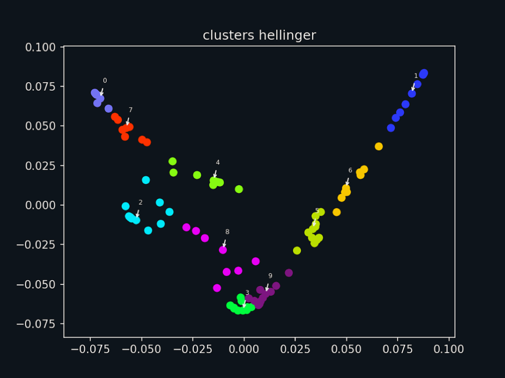
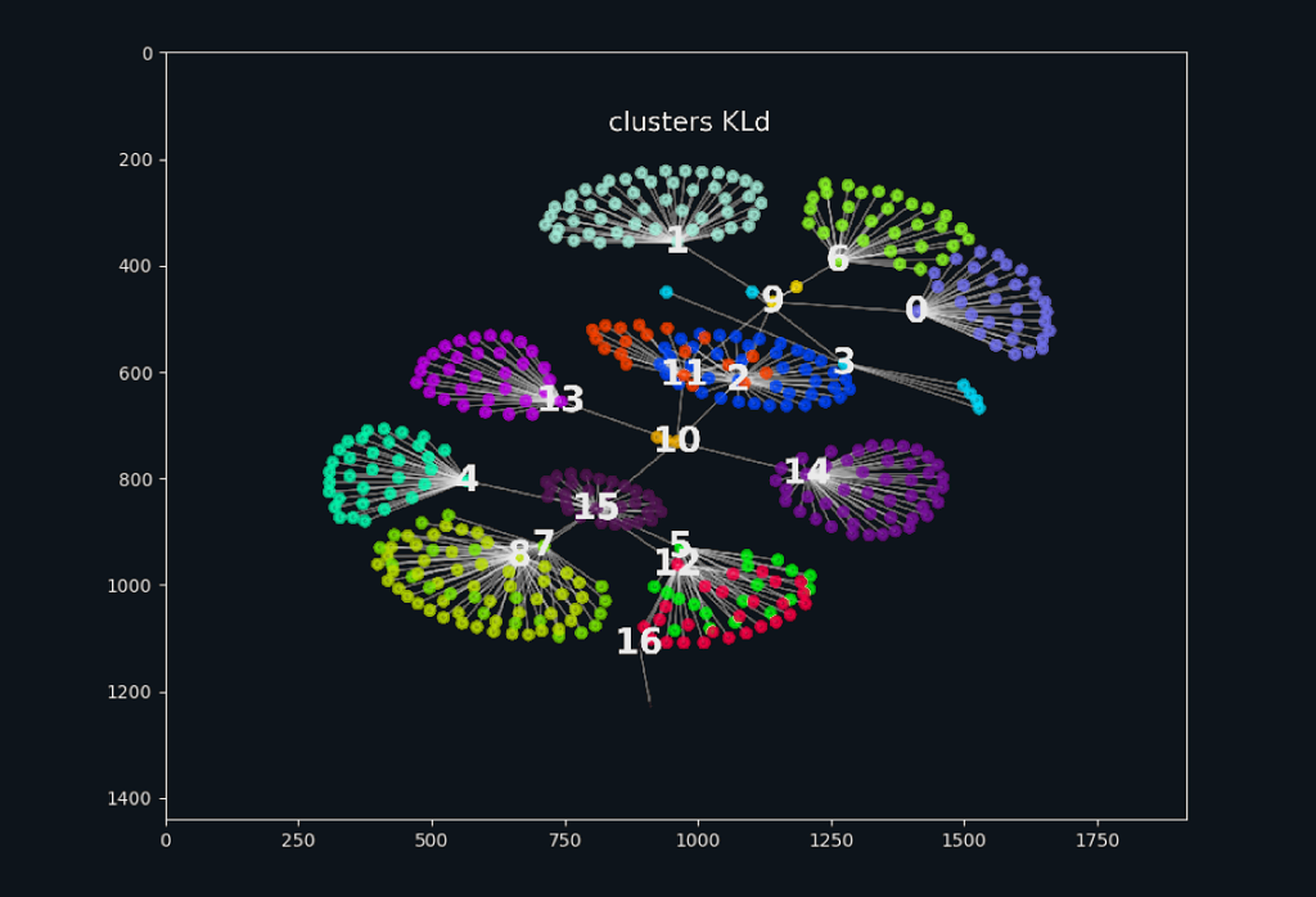
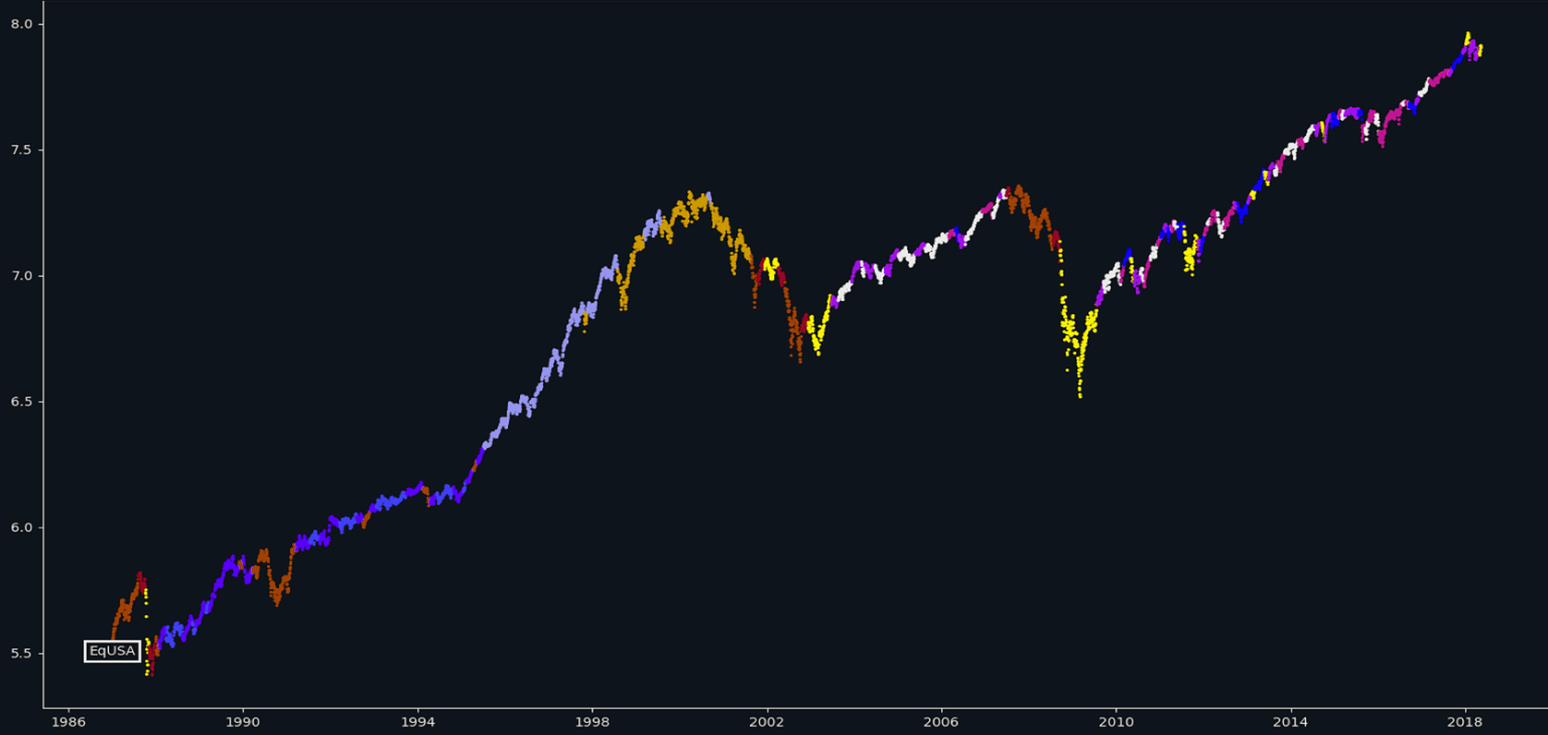
Clustering market states

Regime sequence over time — Regime sequence

// Risk

Vanishing diversification

›Assume assets $Y_1,\dots,Y_m$ follow a mixed joint distribution $P = \pi_1 P_1 + \dots + \pi_q P_q$ , with $\pi_1 > \dots > \pi_q$ .
›Fat tails can be measured as the ratio of risk under $P_1$ to risk under the other regimes.
›An optimizer that accounts for only some regimes reduces risk there but increases it under the others — increasing fat-tailedness.
›Hence regime changes have an aggravated impact on portfolio risk.

// Model

Hidden Markov model & MCMC

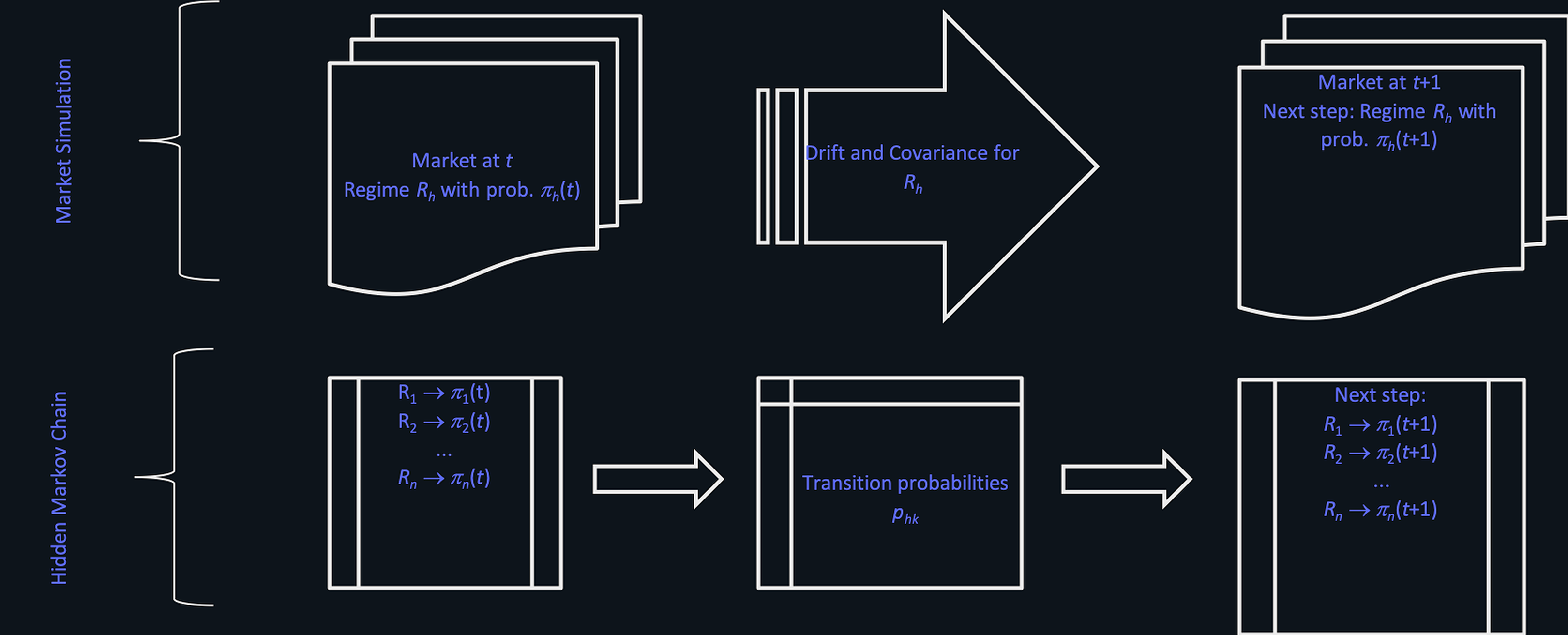
›A finite number of regimes $R_1,\dots,R_m$ , each Gaussian: $R_k \sim \mathcal{N}(m_k, \Gamma_k)$ with drift vector $m_k$ and covariance matrix $\Gamma_k$ .
›A transition matrix $P(t, t+1) = (p_{hk})$ , where $p_{hk}$ is the probability of moving from $R_h$ to $R_k$ ; $\forall h,\ \sum_{k=1}^{m} p_{hk} = 1$ and $P(t, t+n) = P^n$ .
›Euler scheme on $t_0,\dots,t_n$ : pick the next regime $R(t_{i+1})$ by applying $P$ to $R(t_i)$ , then simulate the market under $R(t_{i+1})$ .
›The result is a Gaussian mixture with fat tails, asymptotically Gaussian with $\mu_\infty = \sum_{k=1}^{m} \pi_k \mu_k$ and $\Gamma_\infty = \sum_{k=1}^{m} \pi_k \Gamma_k$ , where $P'\pi = \pi$ , $\pi = (\pi_1,\dots,\pi_m)$ .

Markov chain Monte-Carlo regime transitions — Markov chain Monte-Carlo

// Calibration

From history to regimes

01Find breakpoints $t_1,\dots,t_n$ that split history into homogeneous periods $J_k = [t_{k-1}, t_k]$ .
02Calibrate a Gaussian $\mathcal{N}(\mu_k, \Gamma_k)$ on each period $J_k$ .
03Cluster the set $\Phi = \{(\mu_k, \Gamma_k)\}$ using an information distance (Kullback-Leibler, Tsallis, Hellinger…).
04These live in $n(n+3)/2$ dimensions, so they never recur: describe the market with fewer indices and project $\Phi_k$ with spectral embedding, approximately preserving distances, until recurrence appears.
05Estimate transition probabilities — SVM or EM are more accurate than Baum-Welch, and depend on time spent in a regime.
06Crisis prediction: flag a mild regime that is likely to transition to a wild one.

// Validation

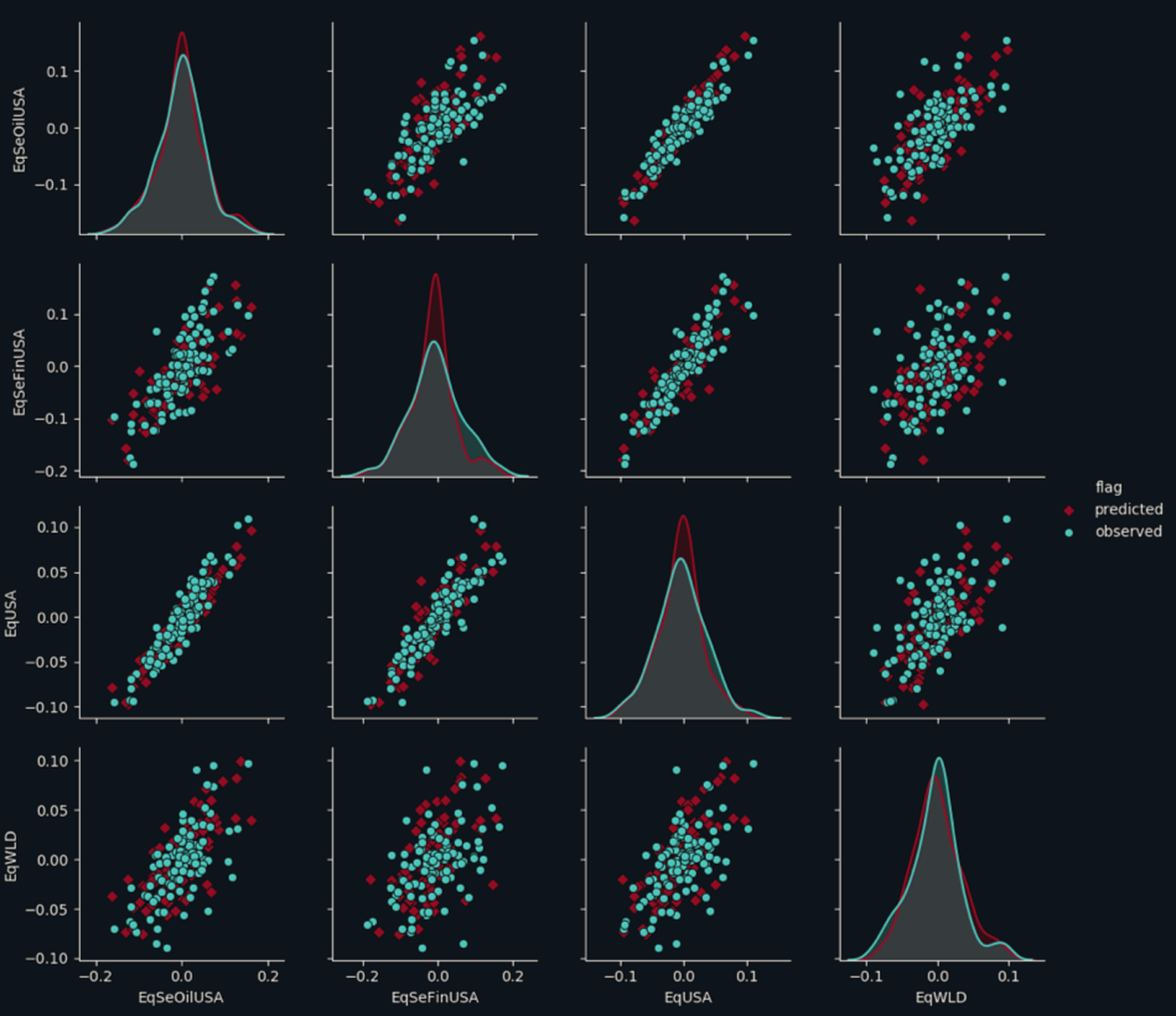
Simulation vs. observed